Opensourceの有限要素法ベースのCFDソルバーであるFEniCSを使ってみようと思い最近触り始めました.
WSLとanacondaを用いてFEniCSのインストールを行いました.
開発環境はWSL+anaconda+jupyter notebookです.
↓インストールの詳細に関しては以下の記事を参照しました.
今回は有名なカルマン渦列のシミュレーションを行います.
↓カルマン渦列です(日本機械学会より引用https://www.jsme.or.jp/jsme-medwiki/09:1002355).

チュートリアルでカルマン渦列のシミュレーションをしようとしたのですがエラーが多く思うように動作しません.
↓参考にしたチュートリアルの記事
記事中ではFenicsの内部関数で形状・メッシュの作成を行っていましたが,以下のようなエラーが出て動きませんでした.
---------------------------------------------------------------------------
ImportError                               Traceback (most recent call last)
/tmp/ipykernel_9077/1743617236.py in <module>
----> 1 import mshr

~/anaconda3/lib/python3.8/site-packages/mshr/__init__.py in <module>
     22 import dolfin
     23
---> 24 from .cpp import Circle
     25 from .cpp import Ellipse
     26 from .cpp import Rectangle

ImportError: generic_type: type "CSGGeometry" referenced unknown base type "dolfin::Variable"
↓FEniCS projectのオープンスラックで質問したところ以下のような回答が得られました.
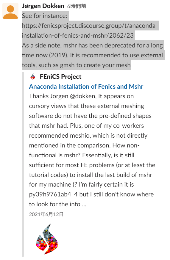
どうやら,FEniCS内部で形状とメッシュを作成するmshrは非推奨となっているようです.外部のメッシャーで構築したメッシュをFEniCS内部に読み込むということでしょうか.
今回は面倒だったのでカルマン渦用のメッシュをgithubから拾ってきました.このリポジトリ内のdolfin/data/meshes/内のcylinder.xml.gzを使用します.
↓動作を確認したコードを以下に貼っておきます.
from dolfin import *

# Print log messages only from the root process in parallel
parameters["std_out_all_processes"] = False;

T = 5.0            # final time
num_steps = 5000   # number of time steps
dt = T / num_steps # time step size
mu = 0.001         # dynamic viscosity
rho = 1            # density

mesh = Mesh("cylinder.xml.gz")

# Define function spaces
V = VectorFunctionSpace(mesh, "Lagrange", 2)
Q = FunctionSpace(mesh, "Lagrange", 1)

# Define boundaries
inflow   = 'near(x[0], 0.0)'
outflow  = 'near(x[0], 2.4)'
walls    = 'x[1]<0.0 || near(x[1], 0.4)'
cylinder = 'on_boundary && x[0]>0.1 && x[0]<0.3 && x[1]>0.1 && x[1]<0.3'

# Define inflow profile
inflow_profile = ('4.0*1.5*x[1]*(0.41 - x[1]) / pow(0.41, 2)', '0')

# Define boundary conditions
bcu_inflow = DirichletBC(V, Expression(inflow_profile, degree=2), inflow)
bcu_walls = DirichletBC(V, Constant((0, 0)), walls)
bcu_cylinder = DirichletBC(V, Constant((0, 0)), cylinder)
bcp_outflow = DirichletBC(Q, Constant(0), outflow)
bcu = [bcu_inflow, bcu_walls, bcu_cylinder]
bcp = [bcp_outflow]

# Define trial and test functions
u = TrialFunction(V)
v = TestFunction(V)
p = TrialFunction(Q)
q = TestFunction(Q)

# Define functions for solutions at previous and current time steps
u_n = Function(V)
u_  = Function(V)
p_n = Function(Q)
p_  = Function(Q)

# Define expressions used in variational forms
U  = 0.5*(u_n + u)
n  = FacetNormal(mesh)
f  = Constant((0, 0))
k  = Constant(dt)
mu = Constant(mu)
rho = Constant(rho)

# Define symmetric gradient
def epsilon(u):
    return sym(nabla_grad(u))

# Define stress tensor
def sigma(u, p):
    return 2*mu*epsilon(u) - p*Identity(len(u))

# Define variational problem for step 1
F1 = rho*dot((u - u_n) / k, v)*dx  + rho*dot(dot(u_n, nabla_grad(u_n)), v)*dx  + inner(sigma(U, p_n), epsilon(v))*dx  + dot(p_n*n, v)*ds - dot(mu*nabla_grad(U)*n, v)*ds  - dot(f, v)*dx
a1 = lhs(F1)
L1 = rhs(F1)

# Define variational problem for step 2
a2 = dot(nabla_grad(p), nabla_grad(q))*dx
L2 = dot(nabla_grad(p_n), nabla_grad(q))*dx - (1/k)*div(u_)*q*dx

# Define variational problem for step 3
a3 = dot(u, v)*dx
L3 = dot(u_, v)*dx - k*dot(nabla_grad(p_ - p_n), v)*dx

# Assemble matrices
A1 = assemble(a1)
A2 = assemble(a2)
A3 = assemble(a3)

# Apply boundary conditions to matrices
[bc.apply(A1) for bc in bcu]
[bc.apply(A2) for bc in bcp]

# Create XDMF files for visualization output
u_file = File('navier_stokes_cylinder/velocity.pvd')
p_file = File('navier_stokes_cylinder/pressure.pvd')

# Create time series (for use in reaction_system.py)
timeseries_u = TimeSeries('navier_stokes_cylinder/velocity_series')
timeseries_p = TimeSeries('navier_stokes_cylinder/pressure_series')

# Save mesh to file (for use in reaction_system.py)
File('navier_stokes_cylinder/cylinder.xml.gz') << mesh

# Time-stepping
t = 0
for n in range(num_steps):

    # Update current time
    t += dt

    # Step 1: Tentative velocity step
    b1 = assemble(L1)
    [bc.apply(b1) for bc in bcu]
    solve(A1, u_.vector(), b1, 'bicgstab', 'hypre_amg')

    # Step 2: Pressure correction step
    b2 = assemble(L2)
    [bc.apply(b2) for bc in bcp]
    solve(A2, p_.vector(), b2, 'bicgstab', 'hypre_amg')

    # Step 3: Velocity correction step
    b3 = assemble(L3)
    solve(A3, u_.vector(), b3, 'cg', 'sor')

    # Plot solution
    plot(u_, title='Velocity')
    plot(p_, title='Pressure')

    # Save solution to file (XDMF/HDF5)
    u_file << u_
    p_file << p_

    # Save nodal values to file
    timeseries_u.store(u_.vector(), t)
    timeseries_p.store(p_.vector(), t)

    # Update previous solution
    u_n.assign(u_)
    p_n.assign(p_)

    # Update progress bar
    print('u max:', u_.vector().get_local().max())
細かいコードの解釈はまだできていないため,今後解釈でき次第追記していきたいと思います!
可視化はおなじみのParaviewで行いました.
↓カルマン渦列が見えますね!

見知らぬ人が作成したメッシュなのでかなり荒いメッシュです.
今度は自力でメッシュ作成からFEniCSで流体計算までしてみようと思います!